Direct integration, also known as symbolic or analytical integration, involves finding an antiderivative or primitive function that represents the area under a curve. However, in many real-world scenarios, the function we're trying to integrate might not have a simple antiderivative or might be too complex to integrate symbolically. In such cases, numerical methods come to the rescue.

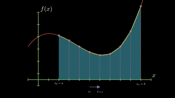
Numerical integration methods provide approximate solutions to definite integrals by breaking down the area under the curve into smaller, more manageable shapes like rectangles, trapezoids, or parabolas. By summing up the areas of these shapes, we can get an approximation of the total area under the curve.

Step Size (h):

$$h = \frac{b-a}{n}$$

$$ n = number \space of \space intervals$$

Try it out:

$$\int_{0}^{1} x^2 \, dx = \left[ \frac{x^3}{3} \right]_0^1 = \frac{1^3}{3} - \frac{0^3}{3} = \frac{1}{3}$$

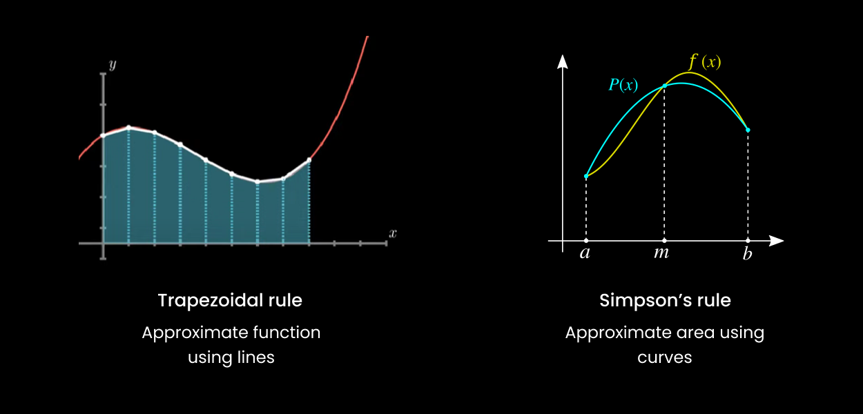
Trapezoidal Rule

This method approximates the area under the curve using trapezoids. The area of each trapezoid is computed and then summed up to get the total area.

Main Idea: Divide the interval into smaller subintervals and approximate the area under the curve using trapezoids over each subinterval.

Visualization:

Equation:

$$I(h) = h \times (\frac {y_0 + y_n}{2} + y_1 + y_2 +...)$$

Code:

#include <bits/stdc++.h>
using namespace std;
double f(double x) {
// Example function, you can replace this with any function
return x*x; 
}
double trapezoidalRule(double a, double b, int n) {
    double h = (b - a) / n;
    double result = 0.5 * (f(a) + f(b));

    for (int i = 1; i < n; i++) {
        result += f(a + i*h);
    }
    return h * result;
}
int main() {
    double a = 0.0, b = 1.0; // Integration limits
    int n = 100; // Number of subintervals
    cout << "Approximate value of integral: " << trapezoidalRule(a, b, n) << std::endl;
    return 0;
}

Simpsons 1/3 Rule

This method uses parabolas to approximate the area under the curve.

Main Idea: Use quadratic polynomials to approximate the function over pairs of subintervals.

Visualization:

Equations:

$$I(h) = \frac{h}{3} \times ((y_0 + y_n) + 4(y_1 + y_3 + ..) + 2(y_2 + y_4 + ...))$$

Code:

double simpsonsOneThirdRule(double a, double b, int n) {
    double h = (b - a) / n;
    double result = f(a) + f(b);

    for (int i = 1; i < n; i++) {
        if (i % 2 == 0) {
            result += 2 * f(a + i*h);
        } else {
            result += 4 * f(a + i*h);
        }
    }
    return (h / 3) * result;
}

Simpsons 3/8 Rule

This method is an extension of Simpson's 1/3 rule and uses cubic polynomials for approximation.

Main Idea: Use cubic polynomials to approximate the function over sets of three subintervals.

Visualization:

Equation:

$$I(h) = \frac{3h}{8} \times ((y_0 + y_n) + 3 (y_1 + y_2 + y_4 + ..) + 2(y_3 + y_6 + ..) )$$

Code:

double simpsonsThreeEighthRule(double a, double b, int n) {
    double h = (b - a) / n;
    double result = f(a) + f(b);

    for (int i = 1; i < n; i++) {
        if (i % 3 == 0) {
            result += 2 * f(a + i*h);
        } else {
            result += 3 * f(a + i*h);
        }
    }

    return (3 * h / 8) * result;
}

Difference between Trapezoidal and Simpson's method

Romberg Integration

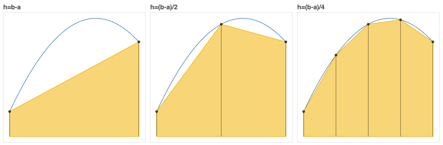
Romberg Integration is a powerful numerical integration method that combines the trapezoidal rule with Richardson extrapolation to achieve faster convergence and higher accuracy.

Main Idea: Romberg Integration starts with the trapezoidal rule and then refines the approximation using Richardson extrapolation. The method takes advantage of the fact that the error in the trapezoidal rule can be expressed as a power series in the step size. By computing the trapezoidal rule for different step sizes and combining the results, the leading error terms can be eliminated, leading to a more accurate approximation.

Details:

1. Initialization: Start with the coarsest approximation using the trapezoidal rule over the entire interval [a,b].

2. Refinement: Halve the step size and compute the trapezoidal rule again. This gives a finer approximation.

3. Richardson Extrapolation: Use the coarse and fine approximations to compute a new, even more accurate approximation. This is done by eliminating the leading error term.

$$f'(x) = \frac{D(rh)-D(h)r^2}{1-r^2}$$

$$D(h) = \frac{f(x+h) - f(x-h)}{2h}$$

1. Iteration: Repeat the refinement and extrapolation steps until the desired level of accuracy is achieved or a maximum number of iterations is reached.

Visualization:

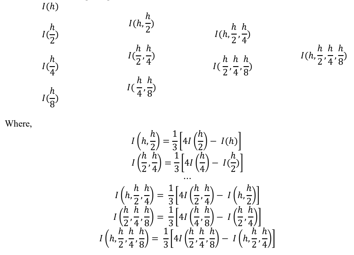
The tabular method for calculating Romberg's approximation using h, h/2, h/4, h/8:

Code:

double rombergIntegration(double a, double b, int n, int m) {
    double h = (b - a) / n;
    double R[n+1][m+1];

    for (int i = 0; i <= n; i++) {
        R[i][0] = 0.5 * h * (f(a + i*h) + f(b + i*h));
    }

    for (int j = 1; j <= m; j++) {
        h /= 2;
        for (int i = 0; i <= n - pow(2, j-1); i++) {
            R[i][j] = 0.5 * R[i][j-1] + h * f(a + i*h + h/2);
        }
        for (int k = 1; k <= j; k++) {
            R[0][k] = R[0][k-1] + (R[0][k-1] - R[0][k-2]) / (pow(4, k) - 1);
        }
    }

    return R[0][m];
}

Thank you for reading the article!