Popular algorithm and passings for single source shortest path

Three commonly used methods for determining the shortest path from a single starting node require a fundamental understanding of graphs. These algorithms are as follows:
Shortest path in a Directed Acyclic Graph (DAG) using topological sorting
The Dijkstra algorithm
The Bellman-Ford algorithm
Relax Function (Edge Relaxation): (IMPORTANT)
In graph algorithms, particularly shortest path algorithms like Dijkstra's and the Bellman-Ford algorithm, the "Relaxation" process, also known as "Node Relaxation," is a crucial step that helps in finding the shortest paths efficiently.
Relaxation involves optimizing the current known distance to a node by potentially replacing it with a shorter distance. The process compares the distance of a potential path through a neighboring node to the currently known shortest path to the destination node. If the potential path is indeed shorter, the distance of the destination node is updated, and this action is referred to as "relaxing" the edge or the node.
Consider a graph where you are trying to find the shortest distance from a source node to other nodes. During relaxation, if you find a path that is shorter than the currently known path, you update the distance of the destination node with this shorter distance. This process iterates through all the nodes in the graph, ensuring that the distances are accurately updated based on the shortest paths discovered so far.
Algorithm:
relax(i,j,distance[], weight[][]):
if distance[i] + weight[i][j] < distance[j]:
   distance [j] = distance[i] + weight[i][j]
   predecessor [j] = i
end if
Shortest path in a DAG using topological sorting
When dealing with a Directed Acyclic Graph (DAG), a graph without any cycles, we can find the shortest path from a single source node to all other nodes using a combination of topological sorting and edge relaxation. The key insight is that we process nodes in topological order, calculating the shortest distance to each node based on the distances to its incoming neighbors.
0. single_source_shortest_path_dag (source, topolist, weight, adj):
1. for each vertex i in topolist:
2.     distance [i] = INFINITY
3.     predecessor [i] = NULL
4. end for
5. distance[source] = 0
6. for each vertex i in topolist:
7.     for each adjacent vertex j in adj[i]:
8.         relax(i,j,distance,weight)
9.     end for
10. end for
// Now using the distance and predecessor
// we can measure distance from the single source
// and track the path from source to destination
To make a graph topologically sorted, we have used below algorithm:
0. toposort(u):
1. visited[u] = true
2. for all the adjacency vertex i of adj[u]:
3.     if visited [i] is not true
4.         toposort(i)
5.     end if
6. end for
5. insert u in a linkedlist 'topolist' from front
Example:
The source node is r and explores all shortest paths from the source node. Show the tabular passing.
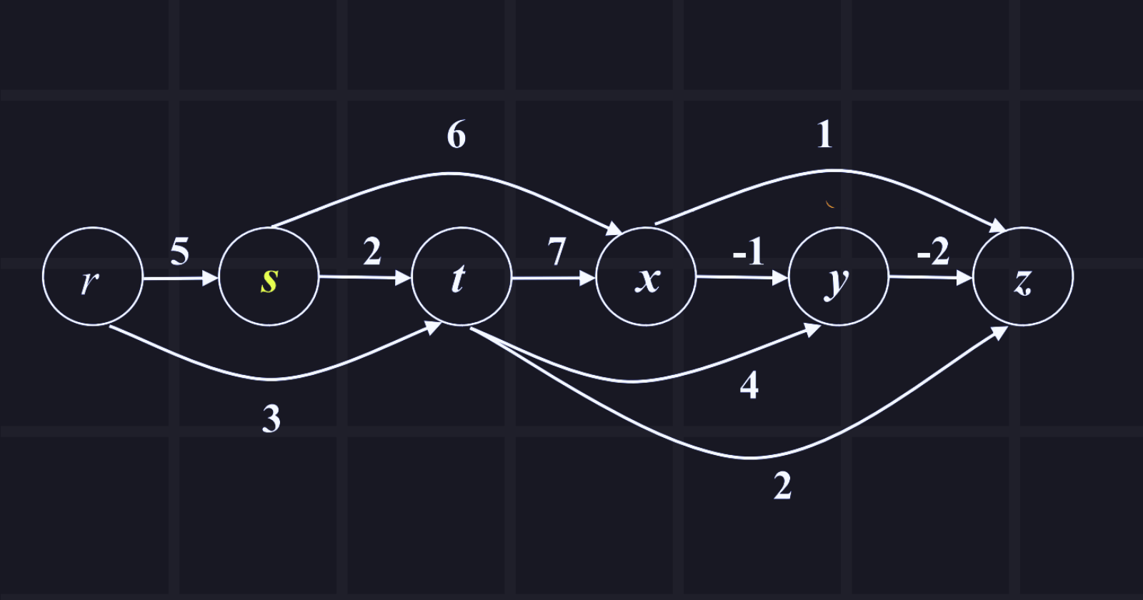
Answer: Tabular passing is given below in the chart,
where distance/pi = cost to reach the node from source node/predecessor's node
| nodes | r | s | t | x | y | z |
| initial | 0/r | INF/NIL | INF/NIL | INF/NIL | INF/NIL | INF/NIL |
| r | 0/r | 5/r | 3/r | INF/NIL | INF/NIL | INF/NIL |
| s | 0/r | 5/r | 3/r | 11/s | INF/NIL | INF/NIL |
| t | 0/r | 5/r | 3/r | 10/t | 7/t | 5/t |
| x | 0/r | 5/r | 3/r | 10/t | 7/t | 5/t |
| y | 0/r | 5/r | 3/r | 10/t | 7/t | 5/t |
| z | 0/r | 5/r | 3/r | 10/t | 7/t | 5/t |
Now, we need to find paths from the source node to other nodes:
r to s: 5 (r -> s)
r to t: 3 (r -> t)
r to x: 10 (r -> t -> x)
r to y: 7 (r -> t -> y)
r to z: 5 (r -> t -> z)
Dijkstra Algorithm
Dijkstra is useful for cyclic non-negative edge graphs where we must find all the shortest paths from a single source node. The algorithm maintains a set of explored nodes and continually updates the shortest distance from the source node to each node in the graph.
Here's the step-by-step description of Dijkstra's algorithm:
Input:
graph: The graph is represented as an adjacency list or matrix.source: The starting node from which to find the shortest paths.
Output:
An array
distanceswheredistances[i]represents the shortest distance from the source node to the nodei.An array
prevwhereprev[i]represents the previous node on the shortest path from the source node to the nodei.Note: To reconstruct the shortest paths themselves, you can use the
prevarray.
Algorithm:
Initialize an array
distanceswith the shortest distance from the source node to each node. Setdistances[source]to 0 and all other distances to infinity.Initialize a priority queue or a min-heap
pqto store nodes and their tentative distances. Add the source node with a distance of 0 topq.Initialize an array
prevto store the previous node on the shortest path for each node.While
pqis not empty: a. Extract the nodeuwith the smallest distance frompq. b. For each neighborvofu:Calculate a tentative distance
new_distancefrom the source tovthroughu. It is the sum of the distance from the source touand the weight of the edge fromutov.If
new_distanceis less than the current distance stored indistances[v], updatedistances[v]withnew_distanceand setprev[v]tou.Add node
vtopqwith its updated distance.
Once the algorithm finishes, the
distancesarray will contain the shortest distances from the source node to all other nodes and theprevarray will allow you to reconstruct the shortest paths.
dijkstra(source, adj):
    distances.assign(N, INF)
    prev.assign(N, -1)
    distances[source] = 0
    prev[source] = source
    pq.push({distances[source], source})
    while pq is not empty:
        u = pq.top().first
        u.pop()
        for all neighbour node v of adj[u]:
            if (distances[u] + weight[u][v] < distances[v]):
                distances[v] = distances[u] + weight[u][v]
                prev[v] = u
                pq.push({distances[v], v})
            end if
        end for
    end while
Example:
The source node is s and explores all shortest paths from the source node. Show the tabular passing.
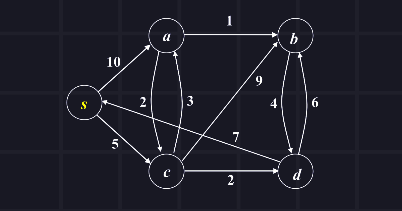
Answer: Tabular passing is given below in the chart,
where distance/pi = cost to reach the node from source node/predecessor's node
| Nodes | s | a | b | c | d |
| initial | 0/s | INF/NIL | INF/NIL | INF/NIL | INF/NIL |
| s | 0/s | 10/s | INF/NIL | 5/s | INF/NIL |
| c | 0/s | 8/c | 14/c | 5/s | 7/c |
| d | 0/s | 8/c | 13/d | 5/s | 7/c |
| a | 0/s | 8/c | 9/a | 5/s | 7/c |
| b | 0/s | 8/c | 9/a | 5/s | 7/c |
Now, we need to find paths from the source node to other nodes:
s to a: 8 (s -> c -> a)
s to b: 9 (s -> c -> a -> b)
s to c: 5 ( s-> c)
s to d: 7 (s -> c -> d)
Bellman-Ford Algorithm
The Bellman-Ford algorithm finds the shortest paths from a single source vertex to all other vertices in a weighted, directed graph. It can handle graphs with negative weight edges and detect the presence of negative weight cycles. This algorithm is named after Richard Bellman and Lester Ford. This algorithm is one of the easiest to find a single source shortest path.
Here's an overview of how the Bellman-Ford algorithm works:
Initialize an array to store the minimum distance from the source vertex to each vertex in the graph. Initially, set the distance to infinity for all vertices except the source, which is set to zero.
Iterate over all edges in the graph repeatedly for a number of times equal to the number of vertices minus one. In each iteration, update the minimum distance to each vertex by considering all possible paths through other vertices.
$$Total\space number\space of \space iteration = Number \space of \space vertex-1$$
After the iteration is complete, check for negative weight cycles. If any vertex's distance can still be improved in one more iteration, it means there is a negative weight cycle in the graph.
If no negative weight cycles are detected, the minimum distances from the source vertex to all other vertices have been computed.
#include <bits/stdc++.h>
using namespace std;

struct Edge {
    int source, destination, weight;
};

void BellmanFord(vector<Edge>& edges, int V, int source) {
    vector<int> distance(V, INT_MAX);
    distance[source] = 0;

    for (int i = 0; i < V - 1; i++) {
        for (const Edge& edge : edges) {
            int u = edge.source;
            int v = edge.destination;
            int w = edge.weight;

            if (distance[u] != INT_MAX && distance[u] + w < distance[v]) {
                distance[v] = distance[u] + w;
            }
        }
    }

    // Check for negative weight cycles
    for (const Edge& edge : edges) {
        int u = edge.source;
        int v = edge.destination;
        int w = edge.weight;

        if (distance[u] != INT_MAX && distance[u] + w < distance[v]) {
            cout << "Graph contains a negative weight cycle!" << endl;
            return;
        }
    }

    // Print the shortest distances from the source vertex
    cout << "Shortest distances from source vertex " << source << ":" << endl;
    for (int i = 0; i < V; i++) {
        cout << "Vertex " << i << ": " << distance[i] << endl;
    }
}

int main() {
    int V, E;
    cout << "Enter the number of vertices and edges: ";
    cin >> V >> E;

    vector<Edge> edges(E);

    cout << "Enter source, destination, and weight for each edge:" << endl;
    for (int i = 0; i < E; i++) {
        cin >> edges[i].source >> edges[i].destination >> edges[i].weight;
    }

    int source;
    cout << "Enter the source vertex: ";
    cin >> source;

    BellmanFord(edges, V, source);

    return 0;
}
Example:
The source node is s and explores all shortest paths from the source node. Show the manual passing. (DO IT BY YOURSELF)
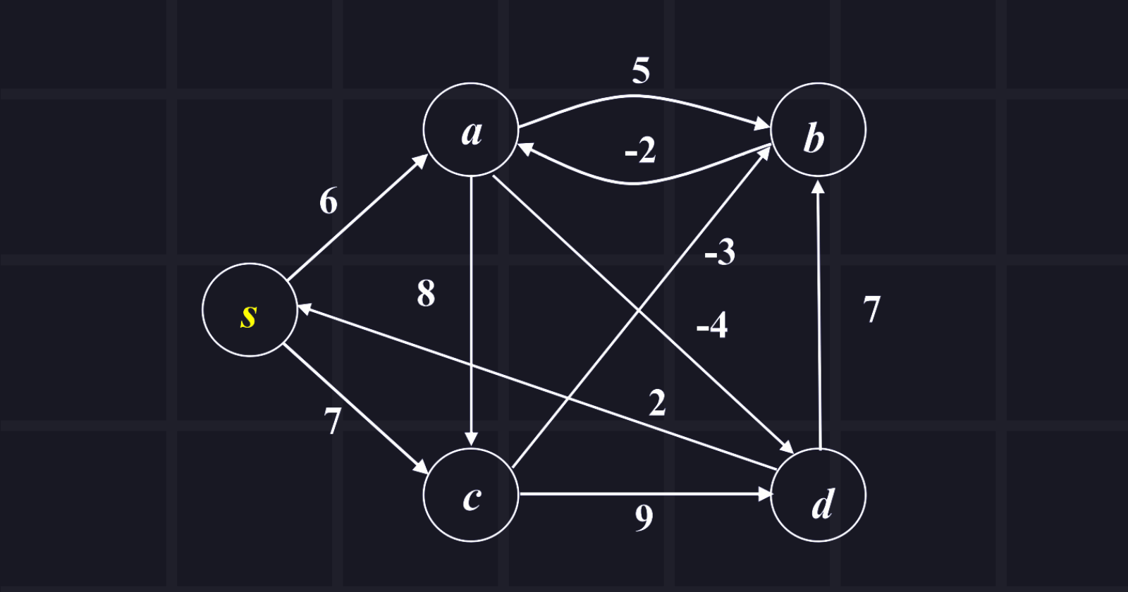
Answer: Passing is given below:
Initial distances:
s = 0
a = Infinity
b = Infinity
c = Infinity
d = Infinity
Edge list:
1. (a, b) = 5
2. (a, c) = 8
3. (a, d) = -4
4. (b, a) = -2
5. (c, b) = -3
6. (c, d) = 9
7. (d, s) = 2
8. (d, b) = 7
9. (s, a) = 6
10. (s,c) = 7
Iteration 1:
Relax edges (s, a) and (s, c).
s = 0
a = 6
b = Infinity
c = 7
d = Infinity
Iteration 2:
Relax edges (a, b), (a, d), and (c, b).
s = 0
a = 6
b = 4
c = 7
d = 2
Iteration 3:
Relax edges (b, a).
s = 0
a = 2
b = 4
c = 7
d = 2
Iteration 4:
Relax edges (a, d).
s = 0
a = 2
b = 4
c = 7
d = -2
Iteration 5:
No relaxes in edge list so it has no negative cycle.
s = 0
a = 2
b = 4
c = 7
d = -2
Note: We can store the predecessor value on edge relaxing updates to get the path.
Here is a table summarizing the differences between DAG shortest path algorithms using topological sort, Dijkstra, and Bellman-Ford:
| Algorithm | Applicability | Time complexity | Can handle negative weights? | Can detect negative weight cycles? |
| DAG shortest path using topological sort | Directed acyclic graphs (DAGs) | O(V + E) | No | No |
| Dijkstra | General graphs | O(E * log V) | No | No |
| Bellman-Ford | General graphs | O(VE) | Yes | Yes |
Thank you for reading the article.